The Arctic is an especially climate-sensitive region of the Earth system, which is evident from the enhanced rate of warming compared to the global average1. In addition to temperature changes, the Arctic has also experienced substantial declines in e.g., sea ice extent, thickness, and concentration2 as well as thawing permafrost3, Greenlandic ice sheet melt4, increasing riverine fresh-water and sediment input into the ocean5, and increasing marine biological activity6. While anthropogenic CO2 emissions are still increasing7, short-lived climate forcers (e.g., black carbon and sulfate aerosols) have been decreasing or plateauing in recent decades8,9. These changes suggest that the anthropogenic influence on Arctic aerosols is decreasing in importance while natural influences on processes affecting aerosols are relatively increasing9. These changes motivate the need to explore the natural components of the Arctic system, especially natural aerosols, which are an important factor in determining the Arctic radiative budget due to their direct and indirect effects10,11. Aerosols are responsible for a large proportion of climate modeling uncertainty12,13,14 and including natural aerosol processes in climate models can help reduce their uncertainty15. Aerosols are expected to respond to the changes in the Arctic environment but determining the direction and magnitude of this response is complex16,17,18. Therefore, investigations on the role and drivers of natural aerosols in the climate system are crucial for evaluating the effects of climate change in this delicate environment9.
Methanesulfonic acid (MSA) in the Arctic is derived mainly from the oxidation of naturally emitted, marine dimethyl sulfide (DMS)19. While the open ocean is the major source of DMS emissions, other sources can contribute as well such as melt ponds, biomass burning, coastal tundra, and lakes20,21,22. DMS is produced from the enzymatic cleavage of dimethylsulfoniopropionate23,24 and represents the largest source of marine biogenic sulfur in the atmosphere25,26. DMS mixing ratios follow a seasonal cycle with near-zero values during polar night (October to February) and elevated and highly variable values during polar day (March to September), typically ranging between 30 and 180 parts per trillion by volume (pptv) for monthly averages21,27,28,29,30,31. Once ventilated into the atmosphere, DMS is oxidized by OH, O3, NO3, and halogens, a process that proceeds via either the addition or abstraction pathways, which are temperature dependent19. In the atmosphere, DMS has a lifetime of approx. 1–2 days21, which is dependent on latitude in the Arctic32. Gas-phase DMS oxidation ultimately yields MSA or SO2 (which is further oxidized to sulfuric acid), with the addition pathway resulting in higher yields of MSA33. DMS can also be oxidized in the aqueous phase (through processing in clouds or on deliquesced particles34) mainly via O3 and OH, which has been demonstrated through modeling and measurements to be an important formation mechanism35,36,37,38,39,40. After dissolving into a droplet, DMS is oxidized into MSA through multi-phase chemistry and during droplet evaporation, MSA is released into the gas-phase and can further influence secondary aerosol production37,39,40. Particulate MSA also follows a seasonal cycle with near-zero values during polar night and elevated values during polar day41,42,43,44. Peak MSA concentrations are experienced during May (~10–40 ng m−3) and typically remain elevated until the end of summer (the seasonal cycle of MSA will be discussed in Section “Seasonal cycle and source regions of Pan-Arctic MSA”). Trends in MSA have shown high spatial and temporal variability in the Arctic, for instance, MSA has increased at Utqiaġvik/Barrow during July-September by 2.5% yr−1 over 1998–201745, at Kevo, Finland, MSA has increased during June/July by 0.68% yr−1 over 1964–201046, and at Alert, CA, MSA has shown decreasing trends during the cold and warm periods over 1980-2000 but increased during the warm period over 2000-20098. The variable trends in MSA are likely related to interannual variability in source strength and transport patterns over the different considered periods8,45,47,48. MSA has a lifetime of several days depending on the environmental conditions49. MSA has been observed to reside mainly in the accumulation mode (aerosols with a diameter > 100 nm)50,51,52 although recent observations have indicated MSA to be in the Aitken mode (~25 < diameter < 100 nm) during a formation event53. MSA is removed from the atmosphere via dry and wet deposition (with wet deposition being the most important37) or further oxidized into sulfate in the aqueous phase39.
MSA is an important constituent in the Arctic atmospheric system, as it has mainly been observed to aid in the condensational growth of aerosols, but has also been modeled to participate in the nucleation of new aerosol particles54,55,56. While its role in nucleation has yet to be directly observed in the field57,58, it has been observed in chamber studies59. More importantly, while only representing a fraction of the total aerosol mass, MSA is critical for the growth of particles to cloud condensation nuclei (CCN) sizes31,32,60 thereby affecting cloud microphysical properties such as cloud lifetime, albedo, and precipitation efficiency61,62,63,64. MSA has been shown to selectively condense onto alkaline particles and not acidic or hydrophobic particles in polar regions65,66. The summertime Arctic is characterized by low particle concentrations, and thus an aerosol-sensitive CCN regime67,68,69, therefore, variations in the number concentration of CCN-active aerosols can have a large effect on the radiative balance of clouds12. Understanding the sources and atmospheric drivers of MSA is therefore vital for accurate modeling of the Arctic climate system, given that aerosol-cloud interactions are one of the largest sources of uncertainty in global climate modeling15.
Machine learning (ML) algorithms and models are powerful tools for understanding environmental phenomena since they can account for non-linear, complex relationships from large datasets that simpler analysis methods wouldn’t be able to accommodate. ML has several advantages over numerical models (NMs), namely computational efficiency, flexibility, and the ability to handle complex non-linear tasks70. ML models are data-driven, meaning they rely solely on the explanatory data and not on pre-defined physical equations, which allows them to efficiently capture complex non-linear relationships for many different applications. NMs rely on physical equations, emission inventories, and assumptions that require accurate parameterizations and estimates, thus limiting their flexibility. As NMs increase in their complexity, the computational costs and runtime increase disproportionately therefore capturing complex atmospheric phenomena can become prohibitively computationally expensive. ML is not without its disadvantages, including the need for large amounts of curated training data and the difficulty in interpreting complex models. Efforts are being made to create hybrid ML-NM models that maximize the advantages of both approaches while minimizing their disadvantages. ML has been demonstrated to be effective in the analysis of environmental processes including predicting sea surface DMS concentrations71,72, aerosol-cloud interactions73, CCN concentrations70,74, and global particle number concentrations75. In the Arctic, k-means clustering has been utilized at several sites to understand the dynamics of aerosol particle number size distributions76,77,78,79,80 and their links to environmental conditions (e.g., open water extent, transport patterns) as well as their sources and climate-relevant properties. Song et al. 81 used a random forest regressor to understand the drivers of different aerosol types on Svalbard and found that solar radiation, surface pressure, and temperature were drivers of biogenic-type aerosols. Hu et al. 82 used principal component analysis coupled with a generalized additive model to show the marine and terrestrial influences on isoprene and monoterpene-derived secondary organic aerosols in the Arctic. Overall, this highlights the applicability of ML models to understand atmospheric phenomena and their advantages over NMs.
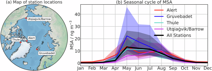
In this study, we leverage in situ observations of particulate MSA from several stations geographically dispersed around the Arctic (Fig. 1a), along with FLEXible PARTicle dispersion model (FLEXPART83) backward dispersion simulations and ERA584 reanalysis meteorological datasets. Our objectives are to (1) identify the Pan-Arctic seasonal cycle and source regions of particulate MSA, (2) elucidate the relationships between MSA and atmospheric variables, and (3) project the future response of MSA based on trends of environmental variables in ERA5. First, we explore the Pan-Arctic seasonal cycles and source regions of MSA. We then use the average trajectory-weighted source regions of MSA and the derived average trajectory-weighted meteorological conditions from ERA5 as input into an ML model and use the SHapley Additive exPlanations (SHAP85) approach for model explainability (see Methods for further details about trajectory-weighted source regions and meteorological conditions as well as SHAP methodology). Following this, we project the future MSA concentrations using the same trained ML model and extrapolated trends in the ERA5 data. We utilize a leave-one-out approach to explore which trends in ERA5 variables are contributing to future changes in MSA. Finally, we discuss the limitations and implications of our results.
Results and discussion
Seasonal cycle and source regions of Pan-Arctic MSA
The seasonal cycle of particulate MSA at each of the four Arctic stations (locations are displayed in Fig. 1a) and for all stations combined, is displayed in Fig. 1b. For a description of each station see the Methods section. For all stations, MSA increases beginning in April and decreases in September, except for Alert which experiences increases beginning in March and decreases beginning in October. This period (April-September) corresponds to polar day, receding sea ice, increase in atmospheric oxidants as well as phytoplankton blooms2,28,86,87. During October-March, MSA is at near-zero concentrations, mainly due to polar night in the Arctic when little biological activity and a minimum of photochemical activity occur26,88. Combining these geographically dispersed stations with their varying seasonal cycles allows us to understand the Pan-Arctic seasonal cycle of MSA as represented by the median of data from all stations (Fig. 1b). Pan-Arctic MSA shows a sharp increase from April to May, stays elevated from May to July (11–13 ng m−3), and gradually decreases until September. This period of elevated MSA during polar day corresponds to enhanced solar radiation and marine biological activity in the Arctic25,26,88. The seasonal cycles presented in this study agree with previous studies which analyzed different periods8,42,47,48. The Pan-Arctic seasonal cycle shows variations from April through September; therefore, we limit our analysis to these months.
The Pan-Arctic seasonal cycle can be attributed to the different geographical locations of each station, as well as varying transport patterns, in relation to biologically active regions of open water. To help contextualize the Pan-Arctic MSA seasonal cycle, the transport climatology was explored for all stations combined for April through September (Fig. 2a). A noticeable feature is the greater geographical extent of air masses during April and September compared to May through August, which is likely a reflection of the extent of the polar dome89,90, which allows for efficient transport from lower latitudes. Whereas during May through August, air masses are mainly confined to marine areas in the Arctic91. It should be noted that the polar dome begins to recede during May, therefore May is often classified as a transition month. Overall, during the peak summer months, air masses mainly arrive from the Greenland/Barents Seas, Baffin Bay/Canadian Archipelago, the Bering Strait/Sea, and the central Arctic Ocean (Fig. 2a).
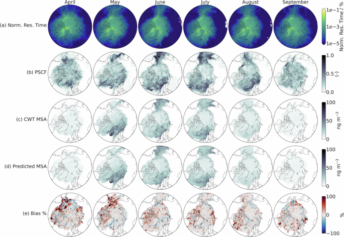
To elucidate the source regions of MSA between April and September, we applied a Potential Source Contribution Function (PSCF) and a Concentration Weighted Trajectory (CWT) analysis using in situ observations of MSA and FLEXPART (see Methods Section for details). Figure 2b and c displays the Pan-Arctic PSCF and CWT, respectively. The PSCF shows the probability for potential source regions, however, it doesn’t show the contribution to observed concentrations that can be expected for a given air mass origin, therefore, we complemented the PSCF with a CWT analysis (Fig. 2c). The PSCF for April shows two regions with a high probability of being source regions, (i) the area extending from the Greenland Sea to lower Baffin Bay, and (ii) continental Alaska. The first area is likely related to the biological activity there6, while the second likely represents transport pathways from the northeastern subarctic Pacific Ocean45,47,71, as observed from May to August (Fig. 2b). During September, the potential source regions of MSA are delocalized around the Arctic. Similar source regions of MSA are observed from May to August (Fig. 2b), which include the Greenland, Barents, Labrador, and Bering Seas. Overall, the marine areas of the Atlantic and Pacific sectors of the Arctic exhibit the highest probability of being an MSA source region during May through July. The CWT analysis supports the PSCF as it shows that the most probable source regions also exhibit the highest contributions to MSA. However, differences exist, for example, during May the PSCF shows that both the Atlantic and Pacific sectors appear to have similar probabilities of being source regions while the CWT shows the Atlantic sector has a higher relative contribution, highlighting the complementary nature of these two approaches. The most probable source regions of the Atlantic and Pacific sectors also make the largest contributions to MSA during the summer, which is likely due to a combination of relatively stronger biological activity and air mass transport from these regions.
Elucidating the relationships between MSA and atmospheric variables
A transport climatology and source region analysis are useful, but they cannot elucidate the relationships between atmospheric variables and observed MSA concentrations. To explore these links, we developed an ML approach to model the trajectory-weighted concentration of MSA (or concentration-weighted trajectory, CWT), we derived the trajectory-weighted meteorological conditions (or meteorological-weighted trajectory, MWT) using FLEXPART and ERA5 to use as input for the machine learning model (See Supplementary Fig. 1 for maps of the MWTs). MWTs consider the average meteorological conditions for the actual location of air masses (using the gridded ERA5 data) and are analogous to our target variable (CWT), thus providing appropriate explanatory variables for our specific ML task and the target variable. Appropriate explanatory variables are important as the prediction efficacy of ML models largely depends on the appropriateness of the explanatory data provided (see Methods for a full description of MWTs and their calculation). The XGBoost library implementing gradient-boosted decision trees was selected among other competing models due to computational efficiency, performance, and high generalization accuracy on many data modeling tasks92. The relevant variables were selected using recursive feature elimination (See Supplementary Fig. 3). The model was optimized using the Optuna93 library, which implements a Bayesian approach to hyperparameter tuning, and the SHAP approach was utilized to explain the model. See the Methods Section for further details about the steps in this methodology.
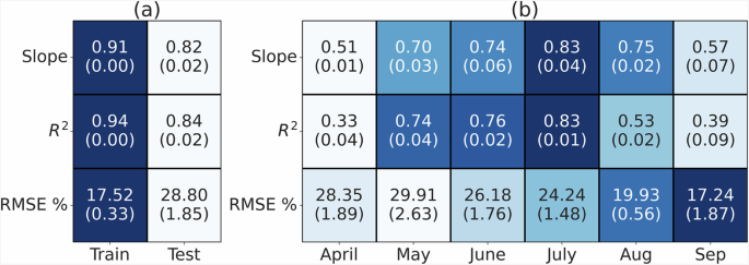
Before interpreting the model results, we evaluate its performance using spatially stratified groups for the training and test sets for all months combined (See Supplementary Fig. 4 for a schematic of the spatially stratified groups) as well as evaluation of the test set on a monthly basis using the slope, R2, and root mean squared error expressed as a percentage of the mean (RMSE %). Figure 3a and b display the results of this model evaluation. The training and test set evaluation shows overall good performance of our model, with a test set mean (±SD) slope and R2 of 0.82 ± 0.02 and 0.84 ± 0.02, respectively, compared to the training set slope and R2 of 0.91 ± 0.003 and 0.94 ± 0.002, respectively (Fig. 3a). These metrics indicate that our model has good performance (high R2/slope and low RMSE % values) and is not strongly overfitting the data (which would be characterized by very high training set metrics and a large difference between training and test set metrics with the latter usually being very poor). When evaluating our model on a monthly basis, we can see that May through August are better reproduced by the model than April and September. Supplementary Fig. 5 shows further investigation of the model performance with boxplots of the percent bias for deciles of the CWT MSA for each month. In this study, bias is defined as the difference between modeled and observed values. A common theme for the distribution of the percent bias in each decile is apparent: at lower values of CWT MSA, the model overpredicts, while at higher values of CWT MSA, the model underpredicts, leading to an overall underestimation of MSA by our model (Fig. 3a). This pattern is also observed when analyzing the spatial bias of our model. Figure 2d and e shows the predicted MSA source regions and the percent bias from the CWT values, which displays this concentration regime bias. It should be noted that the observed CWT MSA is likely biased by the stations being mainly located in the European and North American Arctic (Fig. 1a) and three of the stations experience peak MSA during May and the other in August. There are no long-term observations of MSA in the Siberian Arctic8 and while air masses arriving at these stations cover the entire Arctic area, the Eastern Arctic is likely under-represented in the CWT MSA dataset. Our model overestimates MSA during April/May in the Canadian Archipelago and Alaska, which is likely a result of the low concentrations observed at Utqiaġvik/Barrow during these months (Fig. 2d). These geographic and temporal variabilities should be kept in mind when interpreting the results. Overall, the spatial bias appears to be randomly distributed (with a slight influence from the geography and timing of MSA observations) and the model gives overall satisfactory results, indicating that the model is robust, accurate, and appropriate for the given modeling task.
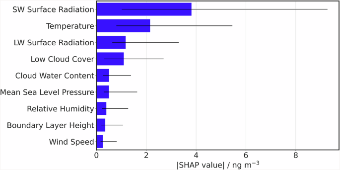
To investigate the drivers of MSA using our model, we used the SHAP methodology which quantifies a variable’s contribution to the model output for a given observation85, whereby variables with positive (negative) SHAP values are actively increasing (decreasing) the model prediction (see Methods for further details). Figure 4 shows the overall variable importance while Supplementary Fig. 6 shows the variable importance on a monthly basis. The overall (or global) variable importance is represented by the median of the absolute SHAP values, with larger values having a greater impact on the model output. It should be noted that the SHAP values do not represent how well these explanatory variables explain the behavior of our target variable in the natural environment but how well these variables explain the behavior of our target variable in our model, therefore representing purely statistical relationships. Given these explanatory variables are environmental data, some correlations between them are unavoidable (Table S3), this can lead to difficulties when explaining the model using the SHAP methodology94. Therefore, to avoid over-interpreting the model results due to correlated variables, we refrain from discussing the rankings of individual explanatory variables but rather discuss which explanatory variables can represent certain processes in the model. From Fig. 4, we can see that the variables with the highest impact on the model are SW radiation, temperature, LW radiation, and low cloud cover, after which the variable importance is low with little variation for the remaining variables. These top four variables are all connected to either the gas- or aqueous-phase oxidation of DMS, which indicates that our model gives physically meaningful and interpretable results. It has been observed before that SW radiation is an important factor connected to MSA81,95,96. SW radiation is necessary for the photochemical production of oxidants (OH, O3, halogens)97, both in the gas- and aqueous-phase, and for stimulating marine biological activity98. SW radiation is therefore expected to have a positive impact on MSA concentrations, indeed MSA is mainly observed during the sunlit, summer months8,47. Temperature affects DMS emission and oxidation to MSA through multiple different mechanisms. Importantly, temperature will affect the sea surface temperature and sea ice extent/concentration, with positive temperatures increasing the DMS emission and reducing sea ice cover26,99,100,101. Temperature would also affect the oxidation of DMS after emission. The gas-phase DMS oxidation produces higher yields of MSA at colder temperatures19,102. The thermodynamic phase of clouds will also be affected by temperature, with positive temperatures indicating the presence of mostly liquid-phase clouds and negative temperatures suggesting mixed- or ice-phase clouds, although this relationship is non-linear103. The thermodynamic phase of clouds would affect the aqueous-phase oxidation of DMS19,36,37,38, with liquid-containing clouds being more efficient than ice-containing clouds. Overall, it appears temperature will have a positive relationship with DMS emission and oxidation to MSA. LW radiation is used here as a proxy for the presence of liquid-containing clouds as liquid cloud water will enhance the downwelling LW radiation compared to clear sky conditions104. While low-level liquid-containing clouds will affect the downwelling LW radiation, other factors including temperature and liquid water content will also have an effect, this should be kept in mind when interpreting the results. Low cloud cover indicates the fraction of low-altitude clouds present although it does not specify the phase (which has implications for the aqueous-phase oxidation of DMS and LW downwelling radiation). The presence of low-level clouds has been demonstrated to aid in the aqueous-phase processing of DMS39,50, although low-level clouds can also reduce the amount of incoming SW radiation. LW radiation and low cloud cover therefore serve as proxies for aqueous-phase processes and are both expected to have an overall positive impact on MSA. These overall top four variables are also consistently amongst the most important variables on a monthly basis (Supplementary Fig. 6), therefore, we will focus our further discussion on these top four variables.
To investigate the relationship of SHAP values between different values of the explanatory variables (explanatory variables refer to variables input into the ML model. i.e., MWTs), we binned the explanatory variables into 10 equally spaced bins and calculated the median and interquartile range of SHAP values for each bin for each month, as displayed in Fig. 5. Supplementary Fig. 7 shows the same figure but including all explanatory variables instead of only the top four. This allows us to discover how certain values of our explanatory variables affect the model output. We also show the geographic distribution of SHAP values for the top four variables and all variables in Fig. 5 and Supplementary Fig. 8, respectively.
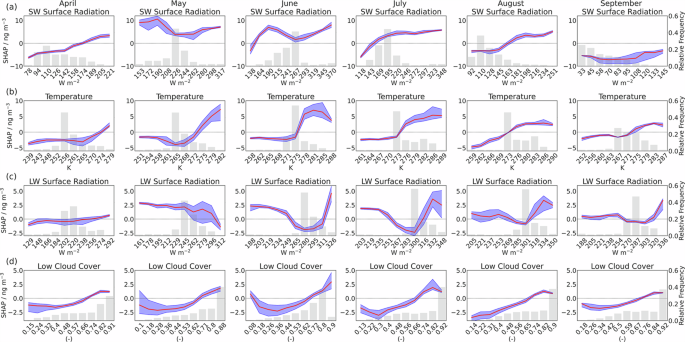
For SW radiation, a complex pattern emerges for the relationship between the explanatory and the SHAP values. During April, July, and August, a mostly linear, monotonic relationship is displayed whilst during May and June a positive, non-monotonic relationship exists (Fig. 5a). During May and September, an entirely positive and negative relationship is observed, respectively. The overall relationship between explanatory and SHAP values of SW radiation supports the postulate that the photo-chemical oxidation of DMS or the production of key oxidants (OH, halogens, or O3, within the aqueous phase or transferred to afterward) is a key atmospheric process leading to the formation of MSA, which is plausible based on theory. Geographically, SW radiation shows ubiquitously positive SHAP values over the Arctic region during May through July and mainly negative SHAP values during April, August, and September (Fig. 6a), corresponding to the seasonal cycle of SW radiation from ERA5 (Supplementary Fig. 2).
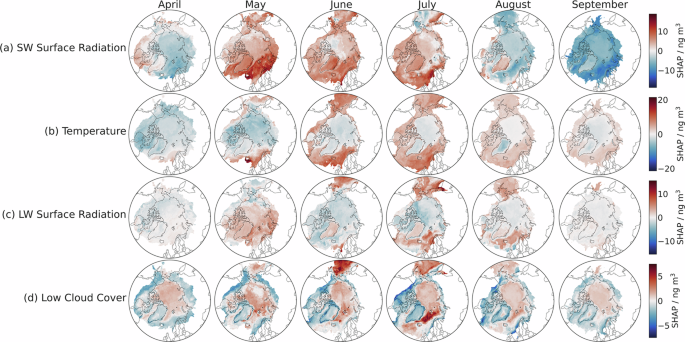
For temperature, during each month the overall relationship between the explanatory and SHAP temperature values is non-linear and there appears to be a threshold value of ~273 K, where afterwards SHAP values turn positive. Below this value, the average temperature SHAP values are all negative and mainly show a flat relationship with temperature values (Fig. 5b). This indicates that areas with above-freezing temperatures will make a positive contribution to the model output of MSA and areas with below-freezing temperatures will make a negative contribution. This is likely related to areas of open ocean with no sea ice, as melting sea ice regulates the overlying atmospheric temperature to around 273 K, thus areas with no sea ice can regularly experience above-freezing temperatures, whereas areas with melting sea ice in the summer experience temperatures around freezing. The absence of sea ice also allows for the emission of DMS into the atmosphere22,105. Song et al. 81 observed an opposite relationship between biogenic type aerosols (which were characterized by high fractions of MSA) and temperature, with a positive impact from temperature up until 273 K and a negative impact afterwards81, suggesting above-freezing temperatures would act to decrease MSA. This pattern was attributed to the role of disappearing sea ice with positive temperatures (which likely serves as a habitat for sympagic algae106) rather than the temperature-dependent kinetics of DMS oxidation. It should be noted that Song et al. 81 was only for a single year (2015) and used in situ measurements of temperature (representative of the conditions at the measurement location) as opposed to spatially-resolved temperature as in this study (representative of conditions in source regions and transport pathways), which would affect the interpretations. Studies from Utqiaġvik/Barrow show positive relationships between MSA and air temperature45. Above-freezing temperatures will also affect the sea surface temperature, the stability of the boundary layer, and the presence of liquid-containing clouds. While the gas-phase oxidation of DMS into MSA has been shown to proceed at faster rates under colder temperatures19,102, the lifetime of intermediates in the aqueous-phase oxidation of DMS into MSA is shorter at warmer temperatures107 and the aqueous-phase oxidation requires the presence of liquid water. Conversely, in areas with below-freezing temperatures, the presence of sea ice (physical barrier to the emission of DMS) as well as mixed-phase clouds (containing ice and supercooled water) is likely negatively affecting this relationship. The geographic distribution of temperature SHAP values closely follows the relationship between explanatory and SHAP values for temperature, with positive SHAP values in regions with positive temperatures (Fig. 6b), which are mainly located at more southerly latitudes. Explanatory and SHAP values for temperature reach their maximum in the marine areas of the Atlantic and Pacific sectors during June and July (Fig. 6b and Supplementary Fig. 1), highlighting the importance of these two regions to MSA formation.
For LW radiation, a different pattern is observed. During April, the contribution of LW radiation to the model output is mostly flat and negative but becomes positive at the highest values. Conversely, during May, a mostly positive contribution from LW radiation is observed which becomes negative at the higher values (Fig. 5c). During June through September, a U-shaped relationship is observed, with a positive contribution from LW radiation at the highest and lowest values, although the most frequent values of LW radiation make a negative contribution. This pattern also suggests that gas- and aqueous-phase processes are both contributing to the model output, with higher values of LW radiation indicating aqueous-phase oxidation and lower values reflecting gas-phase oxidation. Spatially, LW radiation SHAP values show contributions of little magnitude during April and September (Fig. 6c), with slightly positive values in the Atlantic and Pacific sectors and slightly negative over the central Arctic Ocean and continental regions. During May, LW radiation SHAP values are mainly positive geographically except for the Bering Sea region while during June through August, LW radiation SHAP values are positive over the marine areas of the Atlantic and Pacific sectors as well as over the Greenlandic continent (Fig. 6c).
For low cloud cover, the overall relationship is mainly linearly positive and there also appears to be a threshold (~0.7) for positive SHAP values (Fig. 5d). The highest SHAP values are found for the highest values of low cloud cover (which are also the most frequent) and at lower values of low cloud cover, the SHAP values appear to show an increasing tendency (Fig. 5d). This suggests that for low cloud cover both high and low values are contributing to a positive model output of MSA, which also indicates the dual processes of gas- and aqueous phase oxidation of DMS19 during clear and cloudy conditions, respectively, as highlighted for LW radiation. However, it should be noted that the variability of the response for small values of low cloud cover is large (Fig. 5d). For low cloud cover, positive SHAP values are mainly confined to marine areas while continental areas mainly show negative SHAP values. Low cloud cover SHAP values are consistently positive over the central Arctic Ocean, where the MWT is at its highest values (Supplementary Fig. 1). Low cloud cover SHAP values reach a maximum in the Bering Sea during June and in the Greenland/Barents Sea during July (Fig. 6d). The geographic distribution of low cloud cover SHAP values is similar to those of LW radiation, although with noticeable differences which highlights the complementary nature of these two variables as proxies for aqueous-phase processes. LW radiation SHAP values are negative over the central Arctic Ocean while low cloud cover’s SHAP values are mainly positive. This could indicate differences in the cloud phase for this region compared to the marine regions of the Atlantic and Pacific sectors. While low cloud cover indicates that clouds are present, the absence of elevated LW radiation values over the central Arctic Ocean suggests that these clouds are either ice- or mixed-phase clouds, which would emit less LW radiation downwards, as opposed to the more likely liquid-containing clouds in the more southerly regions (Supplementary Fig. 1).
The overall relationships suggest that on average there are two processes making positive contributions to the model output of MSA, gas- and aqueous-phase oxidation of DMS. The positive SHAP values at higher values of SW radiation and lower values of LW radiation suggest that clear sky conditions are also contributing to MSA production through the gas-phase oxidation of DMS. The temperature and low cloud cover threshold values for positive SHAP values as well as the positive SHAP values at higher values of LW radiation (and conversely the negative SHAP values at lower values of SW radiation) indicate that liquid-containing clouds in sufficient amounts are vital for MSA production (i.e., aqueous-phase oxidation of DMS). The model utilized in this study analyzes the geographic and temporal distributions of the explanatory variables based on monthly aggregates, therefore, any temporal information is seasonal and not instantaneous, hence the dual processes identified (gas-phase oxidation in clear conditions and aqueous-phase oxidation in cloudy conditions). This is supported by the relationships observed for other variables. Higher values of total column cloud liquid water and RH both show positive SHAP values (Supplementary Fig. 7), indicating aqueous-phase processes. It should be noted that both these variables are associated with higher uncertainty in ERA5108,109,110. Boundary layer height, wind speed, and mean sea level pressure all show indications of a U-shaped pattern for positive SHAP values (Supplementary Fig. 7). Low values of mean sea level pressure are associated with storms that bring cloudy conditions and high wind speeds (which also increases the boundary layer height and promotes vertical mixing in the ocean surface), these conditions are likely associated with the aqueous-phase processes of MSA production. High values of mean sea level pressure are associated with calm and sunny conditions with low wind speeds, which is likely related to the gas-phase processes contributing to MSA production. Peak MSA concentrations are observed in May (Fig. 1b), therefore, we examined the causes for this peak in more detail (Supplementary Note 1). The peak MSA concentrations in May can be linked to strong marine biological activity and meteorological processes which facilitate the efficient transport from southerly latitudes.
Overall, our model indicates that two main processes are affecting Pan-Arctic MSA concentrations: gas-phase oxidation in clear conditions (indicated through large and mainly positive SHAP values of SW radiation) and aqueous-phase oxidation in cloudy conditions (indicated through U-shaped pattern for LW radiation and low cloud cover values against their SHAP values) which is occurring mainly in the marine areas of the Atlantic and Pacific sectors with temperatures above freezing (threshold for positive temperature SHAP values above 273 K).
Future projections of Pan-Arctic MSA using trends in ERA5 data and machine learning
As discussed in the introduction, MSA concentrations have undergone significant trends, positive and negative, in various parts of the Arctic8,45,46,47,48 and it is plausible that MSA concentrations will change also in the future. Given the relevance of MSA for cloud formation in the Arctic, it is important to understand how the compound might evolve as environmental conditions change in the Arctic.
The ability of our model to represent the seasonal cycle of MSA concentrations and source regions with confidence allows us to project the future response of Pan-Arctic MSA based on past trends of ERA5. We took the entire available record (1979–2022) of the surface level ERA5 variables used in the ML model, aggregated it to monthly means, and performed a trend analysis using the Mann-Kendall/Theil-Sen methodology at a confidence level (CL) of 95% for each month separately (see Methods for further details). Monthly trends for each variable are displayed in Supplementary Fig. 9. The percentage of variables with statistically significant (SS) trends in each grid cell is displayed in Supplementary Fig. 10 which shows that during April and September, most variables are changing in the central Arctic Ocean and during the other summer months the SS trends are more geographically dispersed. Temperature and LW radiation display mainly positive trends during all months and the highest fraction of grid cells with SS trends, wind speed and mean sea level pressure show the lowest fraction of grid cells with SS trends, while all other variables display a mix of positive and negative trends (Supplementary Fig. 10). We project the slope of the trends for SS grid cells forward for different decadal intervals in the future (10 through 50 years in steps of 10 years) and add the total change over a given period to the original value. We assume only SS grid cells will change and the linear trends will continue at the same rate (see Supplementary Note 2 for discussion of limitations and assumptions of this methodology). We use these projected atmospheric conditions to model the future Pan-Arctic MSA, over different decadal intervals up to year 50, using the previously trained ML model. We have constrained these projected atmospheric conditions to physically realistic values (see Table S3 for details on the constraints). Overall, this resulted in a small fraction of data being imputed, which did not significantly affect the results but ensures our projected atmospheric conditions are physically reasonable.
The median and interquartile range of the projected Pan-Arctic MSA concentrations for each month and different decadal intervals is displayed in Fig. 7a. The distributions show slight changes over the decadal intervals, therefore, we tested for SS differences between MSA concentrations for year 0 and each decadal interval. Depending on the properties of the data (normality or homogeneity of variance), either a two-tailed Welsch’s or Student’s t-test was applied on the 95% CL. All of the distributions for each month and decadal interval are significantly different from year 0 (p < 0.05) except for year 10 in May (p = 0.59). The median and interquartile range of the absolute and relative changes in MSA concentrations for each month and decadal interval is displayed in Supplementary Fig. 11. It is evident that there are positive and negative changes in MSA over the entire Arctic. Therefore, we calculated the total relative changes in Pan-Arctic MSA for each decadal interval compared to year 0 (See Methods), the results are displayed in Fig. 7b. The bars and vertical lines represent the total relative changes using the slope and the lower/upper confidence intervals (CIs) from the Theil-Sen estimator, respectively, to project changes in MSA. Two patterns are readily evident from Fig. 7b, first the slightly negative, non-monotonic changes during April and May, and second, the positive, monotonic changes during June through September.
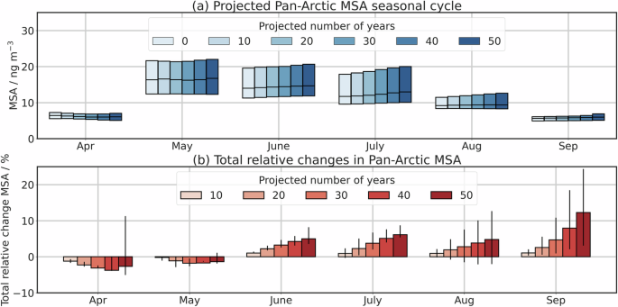
The two patterns presented in Fig. 7b allude to a shift in the seasonal cycle of future projections of Pan-Arctic MSA, with small decreases during the late spring/early summer and larger increases during mid to late summer. Currently, the Pan-Arctic seasonal cycle of MSA peaks during May and stays elevated until July (Fig. 1b), whereas our results postulate that the peak duration of the future seasonal cycle is expected to broaden and the peak month will possibly shift from May to later in the summer. Interannual variation in MSA concentrations is not uncommon in the Arctic8,41,42,43,47, here we project (over long time-scales on the order of decades) that peak Pan-Arctic MSA concentrations will likely undergo a systematic shift to later in the summer although interannual variability is still observed (non-monotonic changes in April/May). The geographic distributions of the changes in MSA reveal that each month experiences both positive and negative changes depending on the geographic location (Supplementary Fig. 12). We focus on the geographic distributions of the year 50 projections as other decadal intervals produce similar patterns but with smaller magnitudes. During April, decreases can be observed over the Arctic Ocean and parts of Siberia while sporadic increases are mainly confined to the periphery of the Arctic, overall the large area with decreases outweighs the sporadic increases. During May, strong decreases are observed in the Greenland, Barents, and Kara Seas as well as the Arctic Ocean, while increases are mainly observed around the southern Greenland, Bering Strait, and the Chukchi Sea. The strong decreases offset the increases to produce an overall decrease during May. During June and July, decreases are mainly confined to the Barents Sea and the northern Pacific Ocean while increases are evident in all other regions, except for the central Arctic Ocean which shows little to no change. During August, decreases are mostly distributed around the marine areas while increases are observed mainly around the Canadian Archipelago and Siberian coast. The Canadian Archipelago is an area where our model overestimates MSA (Fig. 2e) and the increases in this region are likely an upper limit given the overestimation by our model in this region. The low CWT values and presence of model bias in these regions likely contribute to the large CIs for the projections of MSA in Fig. 7b during August. During September, increases are observed mainly in the Greenland Sea region. Interestingly, the regions around Svalbard are experiencing decreases in MSA during all months except for September and the regions around the Bering Strait are mainly experiencing increases during all months (Supplementary Fig. 12). The geographic distribution of the projected changes in MSA is a combination of the trends for each variable and their contribution to the model output in these regions. Overall, while the Pan-Arctic MSA concentrations are projected to change in the future, these changes are heterogeneously distributed geographically.
To elucidate which variables are responsible for the shift in the seasonal cycle, we devised a leave-one-out approach to calculate the contribution of each variable to the projected changes. To inspect the relationship between the trends in a variable and how said variable contributes to the projected changes, we classified each grid cell according to the direction of the trend and contribution. The leave-one-out and classification methodology are described in more detail in the Methods section. The results of the leave-one-out analysis and classification of the year 50 projections are displayed in Fig. 8 and Supplementary Fig. 15, respectively. The effects of the main variables and their trends are summarized in Table 1. During April, positive RH trends are contributing to the projected decrease in MSA. During May and June, increases in MSA due to positive temperature trends are counterbalanced by decreases in MSA due to positive LW radiation trends. During July and August, a more complex picture is presented. For instance, increases in MSA can be attributed to positive LW radiation and negative BLH trends, and decreases in MSA are due to negative SW radiation trends. During September, positive temperature trends are driving the projected increase in MSA, whereas negative low cloud cover trends are contributing to decreases in MSA. Overall, the contribution of a variable and the relationship to said variable’s trends to the projected changes in MSA is highly complex with different variables contributing in different ways in different months. The variables making the highest contribution to projected increases in MSA are temperature, LW radiation, and BLH, while RH, LW, and SW radiation are mainly contributing to the projected decreases in MSA. Of these only BLH and SW radiation show negative trends, highlighting the intricate balance between the (linear) trends of a variable and the (non-linear) relationships with said variable and MSA.
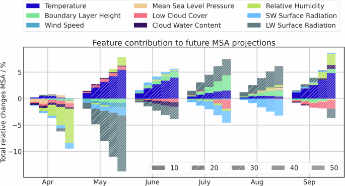
Table 1 Summary of future projections of MSA, which main explanatory variables are contributing to these projections, and how
Atmospheric implications
Changes to the MSA seasonal cycle, as projected by our model, will have an effect on the properties of secondary particles in the Arctic which, in turn, will have direct and indirect implications for the radiative balance. Changes in MSA will affect the physical properties of aerosols, namely mass and volume, which would be especially meaningful during summer and early autumn when total aerosol mass/volume concentrations are at a minimum8,91. The increase in mass/volume will also increase the scattering efficiency, thus having direct implications on the radiative balance. This will also depend on future changes to the underlying surface properties (snow-covered vs bare land or sea ice vs open ocean in a future environment). The changes in MSA concentrations will also likely indirectly affect the aerosol number concentration and therefore CCN concentrations. The additional particulate MSA could affect the number concentration by partitioning into the gas-phase following aqueous-phase formation and droplet evaporation thus providing an additional precursor (or condensable) vapor source. The additional gas-phase MSA could aid in the growth of newly formed particles and possibly participate in nucleation54,55, although this will also depend on changes in sulfuric acid111, iodic acid56,112, and other constituents (e.g., reduced nitrogen compounds and organic acids)113. The number of particles arising from the additional gas-phase MSA that could potentially reach CCN sizes will impact cloud microphysical properties and thus the radiative balance114. This also applies to particles whose hygroscopicity changes from changes in MSA115, as more hygroscopic particles (from additional or less MSA depending on the chemical composition) will more effectively form clouds. These effects would be most pronounced during summer when the sub-micron organic aerosol fraction (which is less hygroscopic) is high44,116,117,118,119, sea salt aerosol is low120, the condensation sink (CS) is lowest, and the cloud regime is CCN-sensitive67. This would also depend on the meteorological conditions (updraught velocities and cloud cover)69 and pre-existing aerosol load in a future environment. Clouds mainly reflect solar radiation during the summer (due to decreases in the underlying surface albedo) and our model projects the largest relative increase in MSA during June and July, therefore, the changes in MSA would likely result in additional negative radiative forcing thus cooling the surface. The changes in MSA could also affect the fate of aerosols. The increase in CCN active particles (either through growth to CCN sizes or changing hygroscopicity in existing particles) will affect the wet removal of the aerosol population. More numerous or more active CCN particles might be preferentially removed via precipitation, therefore even though the source strength is increasing the overall effect on the atmospheric burden might be decreasing, highlighting the complex nature of projecting future changes in aerosol properties9,16,18.
Two important aspects of the environmental system that are pertinent to MSA burdens but are missing from our model are precursor sources (DMS and oxidants) and MSA sinks (wet and dry removal). Studies have shown that in recent decades DMS emission, net primary production, and chlorophyll-α are all increasing in the Arctic6,101,121,122, which could be attributed to a combination of increased open water and nutrient input. Changes in the Arctic ecosystem (shallowing of the oceanic mixed layer depth, increases in sea surface temperature, and acidification)105 will also likely affect the emission of DMS. Geographically, ice break-up, chlorophyll-α, and polar spring blooms are all moving northward123. Biogeochemical modeling studies suggest that under enhanced CO2 levels, DMS emissions will decrease annually overall although with vernal decreases related to increased oceanic mixed layer depth and summer increases due to decreases in sea ice extent124. These studies suggest that not only are sources of DMS strengthening but they are also moving increasingly northward which will positively affect the overall MSA production. Trends in atmospheric oxidants relevant for MSA production indicate that in the Arctic, ozone125,126 and bromine monoxide127 are increasing also. A recent modeling study showed bromine levels are expected to increase in the future due to an increase in first-year sea ice and sea salt aerosol128. Stevenson et al. 129 showed that OH levels are increasing globally and in the Arctic. Together these studies advocate for increasing emission of DMS and atmospheric oxidant levels in the future, both of which will positively affect MSA production. Changes in future precipitation patterns will also affect future MSA concentrations, by physically removing aerosols from the atmosphere but also by lowering the CS for vapors. Using accumulated precipitation along back-trajectories, studies have shown that accumulated precipitation is increasing at two High Arctic sites, mainly during autumn80,130. Interestingly, modeling studies have shown precipitation to increase substantially, especially during summer131,132,133,134. These studies suggest wet removal will become more important in a future Arctic climate and will likely affect our projections of MSA.
Anthropogenic activities (i.e., shipping, tourism, and resource extraction) will also undergo future changes135,136, with predicted increases due to sea ice retreat137,138 and will have an effect on future aerosol and cloud properties139. Increases in anthropogenic activity will likely result in increased emissions of nitrogen oxides (NOx), volatile organic compounds (VOCs), BC, CO, sulfur oxides (SOx), greenhouse gases, and production of O3140. Increased atmospheric burdens of BC and organic aerosol (from VOC oxidation and condensation) from Arctic anthropogenic activities would increase the CS. This would suggest more condensation of MSA onto pre-existing aerosol surfaces rather than contributing to growth of newly formed particles. This would depend on the chemical composition of the coating material and aerosol physicochemical properties65,66. Indeed increased SOx emissions (and thus increased sulfate levels) would increase aerosol acidity thus affecting the partitioning of MSA to the gas-phase following aqueous-phase formation114. Increased levels of NOx and O3 could alter the branching pathways of DMS oxidation to produce more SO2 instead of MSA19,37,96. These changes in the aerosol burden due to anthropogenic activities will in turn affect the Arctic environment, such as increased sea ice/snow melt due to increased BC deposition as well as altered nutrient cycling due to inorganic aerosol deposition. The expected increase of Arctic anthropogenic emissions of CO2 and BC (and reduced emissions of SOx due to regulations) will lead to positive radiative forcing140. These increased emissions will likely have the most impact on local air quality in regions experiencing expanded anthropogenic activities (shipping lanes and areas in proximity to industrial activities) and their overall impact on the aerosol population might be small and will likely have negligible impacts on the radiative budget138. Overall, the increased anthropogenic activity in the Arctic will affect natural aerosol burdens and dynamics, however, how exactly remains elusive.
This analysis shows that the seasonal cycle of the geographic source regions of MSA can be accurately modeled using the average atmospheric conditions and ML, highlighting the potential use of this methodology to be applied to other natural components of the Arctic atmospheric system, i.e., sea salt aerosol and gas-phase DMS. We also provide guidance as to which atmospheric variables are most important for explaining variations in MSA and how, thus emphasizing the need for an accurate representation of the conditions affecting gas- and aqueous-phase oxidation of DMS in chemical transport models. We also show, based only on changes in atmospheric conditions and not changes in oceanic and biological factors affecting DMS emission/oxidation, that MSA is projected to undergo a shift in the seasonal cycle. Other models and observations have shown that these oceanic and biological factors (sea ice extent/concentration, chlorophyll-α, and DMS emissions) are changing over these time ranges, however, precipitation patterns and intensity are also changing. This suggests that changes in oceanic variables will act in conjunction with changes in atmospheric variables to increase Pan-Arctic MSA concentrations although precipitation will likely affect these changes. The competition between source and sink strength will ultimately determine how aerosol components change in the future. How the Arctic environment responds to future climate change (including atmospheric and oceanic conditions) remains an open research question and provides an avenue for future research.